How to Perform Custom Filter in Excel (5 Ways) ExcelDemy
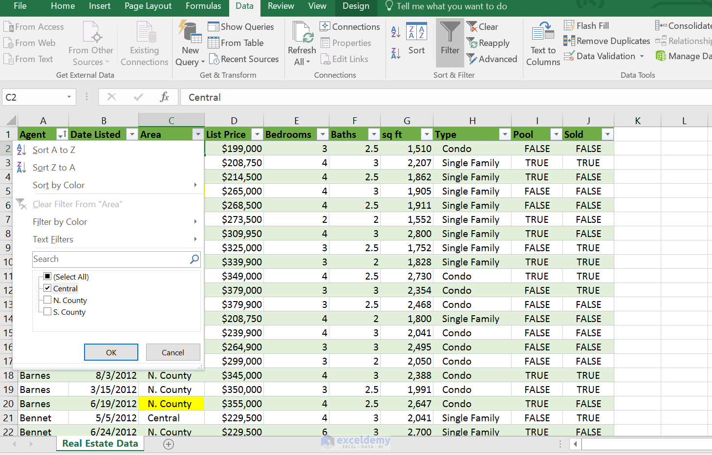
Clear a filter from a column. Click the Filter button next to the column heading, and then click Clear Filter from <"Column Name">. For example, the figure below depicts an example of clearing the filter from the Country column. Note: You can't remove filters from individual columns. Filters are either on for an entire range, or off.
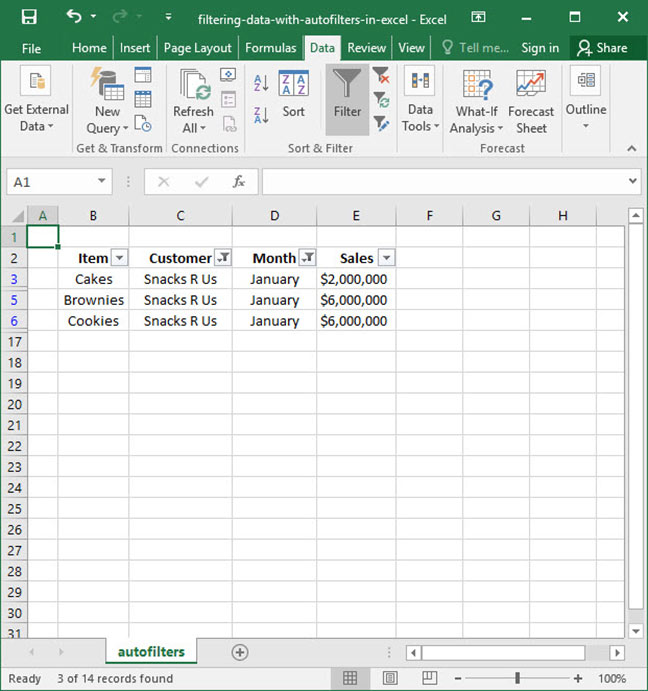
Filtering Data With Autofilters in Excel Deskbright
Example 1 - FILTER returns an array of rows and columns. In this example, cell F3 contains a single formula, but this formula returns an array of values into the neighboring rows and columns. This single formula is returning 2 rows and 3 columns of data where the values in C3-C10 are higher than 100.
How to Filter in Excel CustomGuide
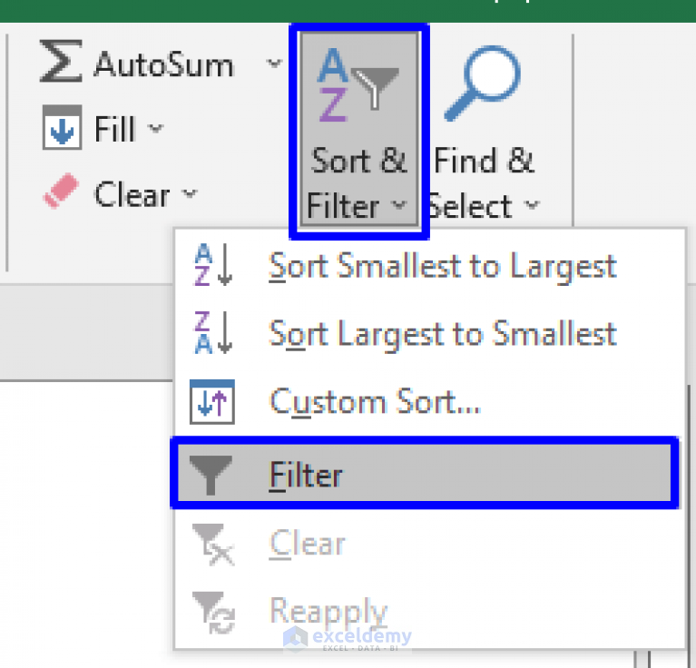
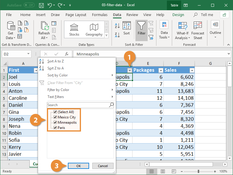
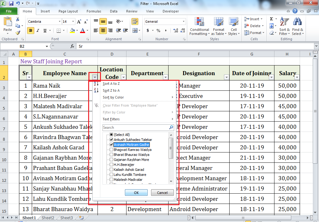
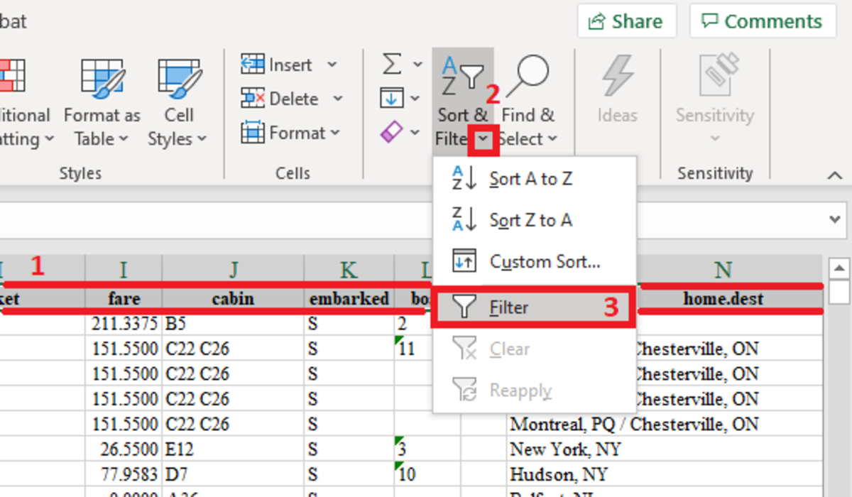
Go to Home > Editing Group > Sort & Filter > Filter. Use the keyboard shortcut to add filters - Control Key + Shift + L. 4. This adds drop-down arrows to the selected column header (Products in this case). 5. The filter is already applied, and you can now use it to filter our information as desired.
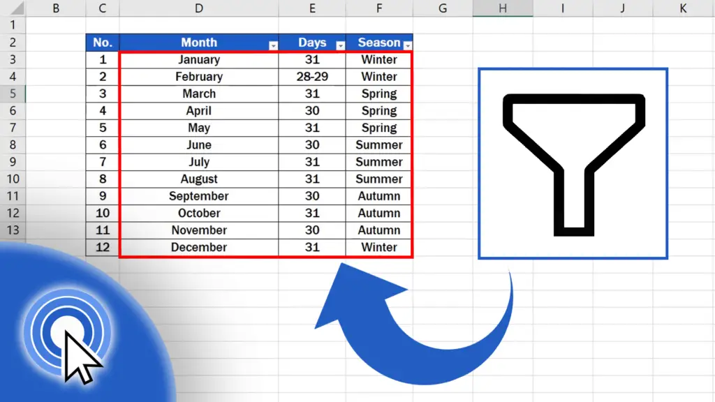
How to Use Sort and Filter with Excel Table ExcelDemy
Daftar Isi Konten: AutoFilter Excel Cara Filter Data Text, Angka, Tanggal dan Warna. #1 AutoFilter Text di Excel. #2 AutoFilter Data Angka di Excel. #3 AutoFilter Tanggal di Excel. #4 AutoFilter Berdasarkan Warna di Excel. #5 Cara Filter Cell Kosong. Cara Hapus Filter Data Excel. Penyebab Filter Excel Tidak Berfungsi.
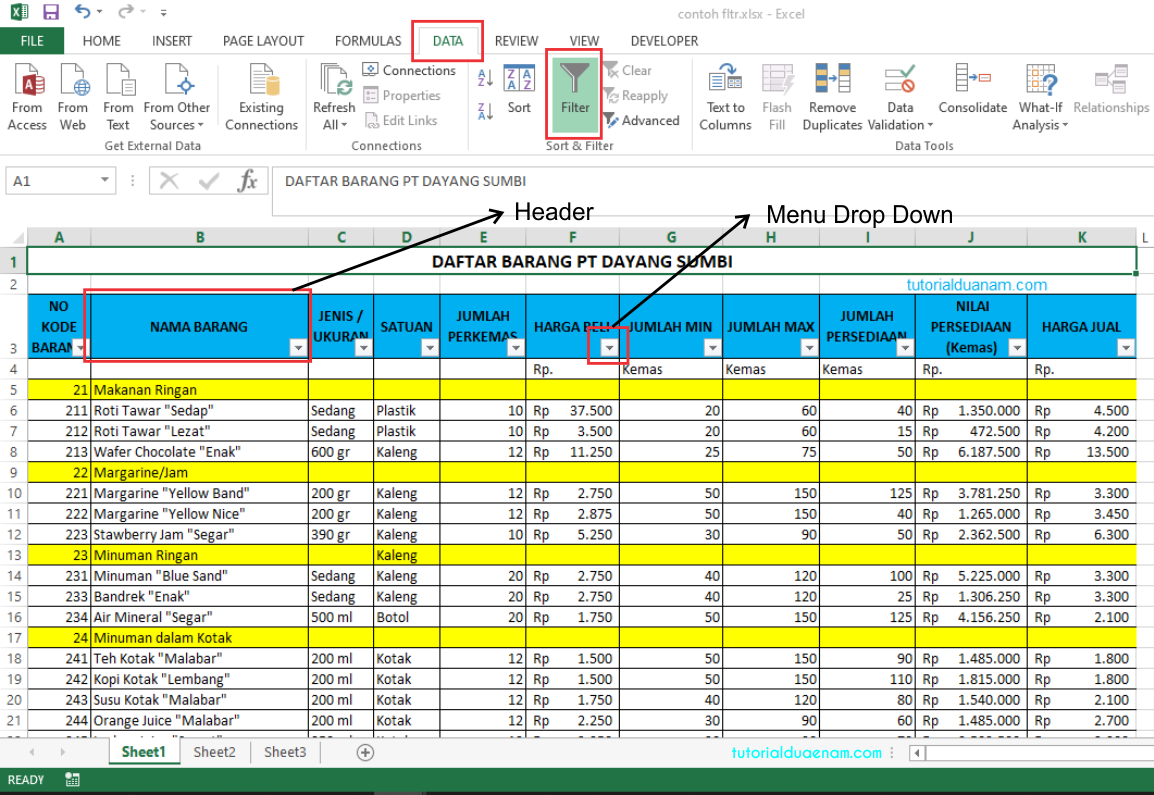
Cara Menampilkan Data Tertentu dengan Fitur Autofilter (Filter) pada Ms. Excel
FILTER based on a list. OK, now it's time to add the FILTER function, using the COUNTIFS as the include argument. The formula in cell I4 is: =FILTER(Data,COUNTIFS(ItemList[Item],Data[Item]),"No values") The previous COUNTIFS formula is highlighted in bold. Only the items from the Data table where the COUNTIFS calculates to 1 or more are retained.
How to Filter in Excel Instructions to Create Filter in 2020
Secara default, memproteksi lembar kerja mengunci semua sel sehingga tidak ada yang bisa diedit. Untuk mengaktifkan beberapa pengeditan sel, selagi membiarkan sel lain terkunci, anda dapat membuka kunci semua sel. Anda hanya bisa mengunci sel dan rentang tertentu sebelum Anda memproteksi lembar kerja dan, secara opsional, memungkinkan pengguna tertentu untuk mengedit hanya dalam rentang lembar.
Excel Functions Data Filter Learn How To Filter Data Of Different Categories And Copy Paste The
3 ways to add filter in Excel. On the Data tab, in the Sort & Filter group, click the Filter button. On the Home tab, in the Editing group, click Sort & Filter > Filter. Use the Excel Filter shortcut to turn the filters on/off: Ctrl+Shift+L.
Using the Excel FILTER Function to Create Dynamic Filters technology for teachers and students
The FILTER function in Excel is used to filter a range of data based on the criteria that you specify. The function belongs to the category of Dynamic Arrays functions. The result is an array of values that automatically spills into a range of cells, starting from the cell where you enter a formula.
How a Filter Works in Excel Spreadsheets
Saat Anda menerapkan ulang operasi filter atau pengurutan, hasil yang berbeda muncul karena alasan berikut: Data telah ditambahkan ke, diubah, atau dihapus dari rentang sel atau kolom tabel. Filter adalah filter tanggal dan waktu dinamis, seperti Hari Ini, Minggu Ini, atau Tahun ke Tanggal. Nilai yang dikembalikan oleh rumus telah berubah dan.

Cara Filter di Excel Terkunci / Filter Excel Protected Sheet YouTube
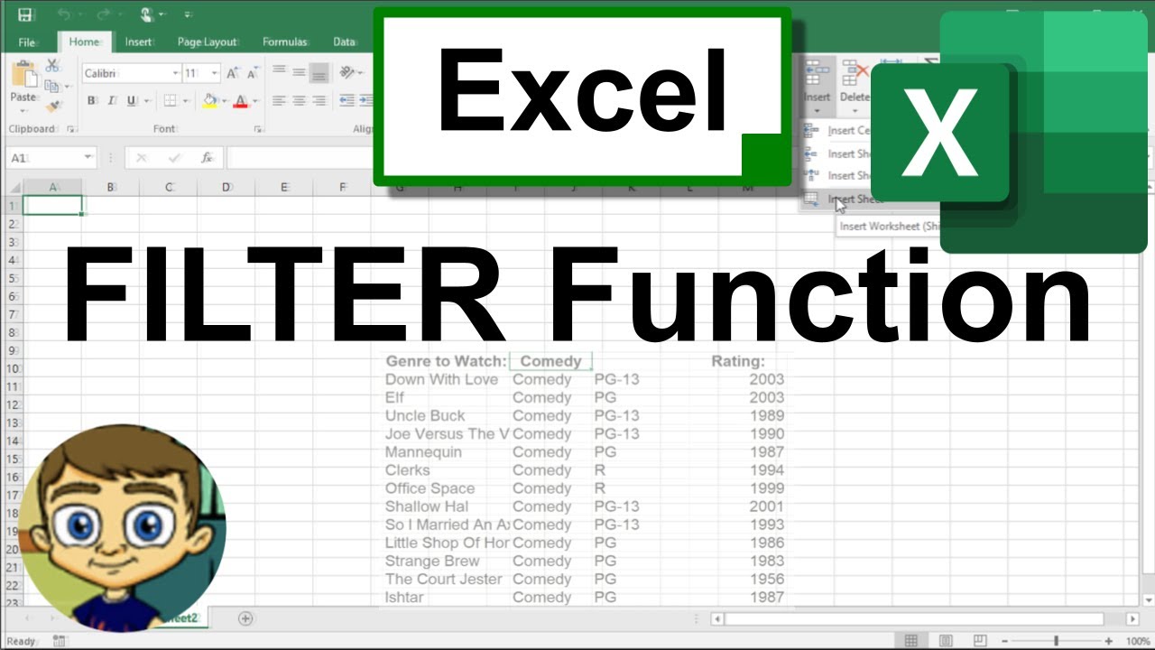
To get started, we'll start with a basic filter so that you can see how the function works. In each screenshot, you'll see our filter results on the right. Related: How to Find the Function You Need in Microsoft Excel. For filtering the data in cells A2 through D13 using the content of cell B2 (Electronics) as criteria, here's the formula:
How to Create Filter in Excel
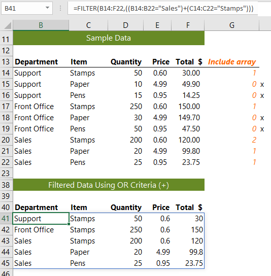
First of all, select cell G5, and write down the FILTER function in that cell. The function will be: =FILTER (B5:B25, (C5:C25="Italy")+ (D5:D25="Italy")) Hence, simply press Enter on your keyboard. As a result, you will get the years when Italy was the host or champion or both which is the return of the FILTER function.
Using the FILTER function in Excel (Single or multiple conditions)
Filtering for Multiple Criteria. Suppose we wish to filter the table for two different criteria: "Game" for the Division and "Asia" for the Region. On the FILTER sheet, select cell G37 and enter "Game" as the comparison value for Division. Select cell G38 and enter "Asia" as the comparison value for Region.
How to Use Excel Filter Function to Analyze Multiple Arrays Tech guide
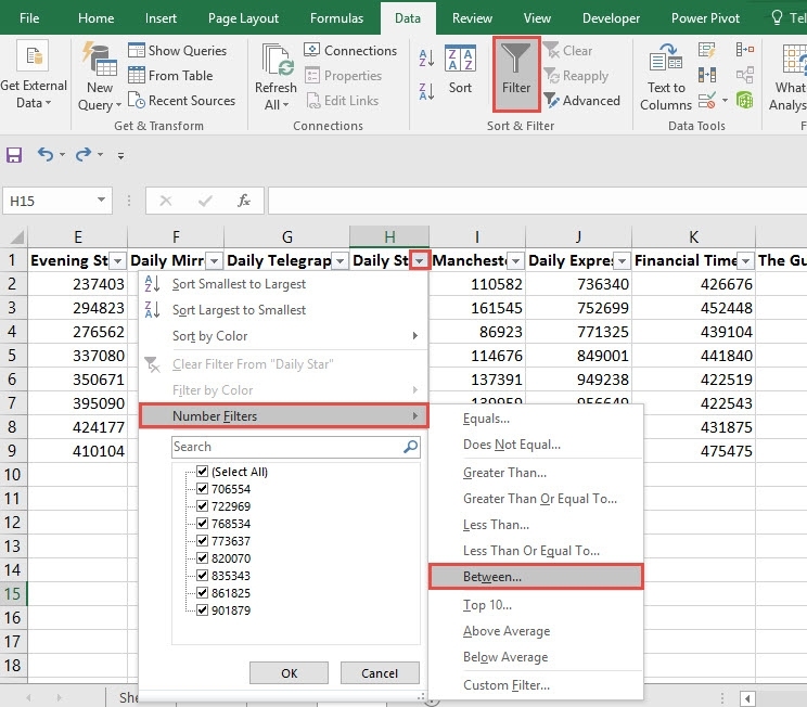
The following are 10 useful keyboard shortcuts to filter data in Excel. 1. Turn Filter / AutoFilter on. To turn Filter on using a keyboard shortcut, ensure a cell in the range is selected and then press Ctrl + Shift + L. If your data range contains any blank columns or rows, select the entire range of cells first.
How to Filter and Sort Data in Microsoft Excel TurboFuture
To filter by using the FILTER function in Excel, follow these steps: Type =FILTER ( to begin your filter formula. Type the address for the range of cells that contains the data that you want to filter, such as B1:C50. Type a comma, and then type the condition for the filter, such as C3:C50>3 (To set a condition, first type the address of the.

How to Use AutoFilter in MS Excel A StepbyStep Guide
Cara Filter di Excel Terkunci / Filter Excel Protected Sheetkita akan membahas bagai mana cara. memfilter di excel meski dalam keadaan terkunci atau ter port.
How to Filter Multiple Rows in Excel (11 Suitable Approaches) ExcelDemy
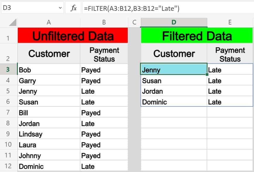
The Excel FILTER function is used to extract matching values from data based on one or more conditions. The output from FILTER is dynamic. If source data or criteria change, FILTER will return a new set of results. This makes FILTER a flexible way to isolate and inspect data without altering the original dataset.